Graph Representation – Quick Tutorial

Graphs are very powerful tools for modeling relations between various entities, with many applications in fields as diverse as physics, biology, networking, natural language processing, etc. In this post we are going to overlook the most common ways of representing graphs in memory.

Graphs are usually defined as an ordered pair G = (V, E) where

• V represents the set of vertices or nodes
• E represents the set of edges, an edge being a link between two vertices

Depending on the problem, a graph or it’s components may have various properties (such as having directed or undirected edges), but every graph implementation should generally provide an implementation for:

• adding a node or an edge
• checking if an edge exists between two nodes
• traversing every edge associated with a node
• (optionally) deleting a node or an edge

There are two common ways to model graphs in memory: using adjacency lists or an adjacency matrix.

Using an Adjacency Matrix

• Building the graph

If we have prior knowledge of the total number of nodes in the graph, building the graph becomes as simple as:

void initGraph(int numNodes) {
     matrix = new boolean[numNodes][numNodes];
     vertices = new Vertex[numNodes];
}

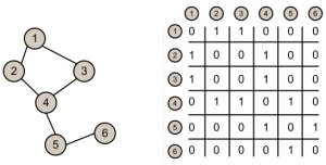
Here matrix[i][j] has the value 1 if there exists an edge from node i to node j and 0 otherwise.

The space required for storing the matrix amounts to Θ (numNodes^2). Depending on usage, we may decide to store additional information for each vertex or edge. For example, here we assume each Vertex object holds an index variable.
Note that, in practice, this representation becomes entirely unfeasible for larger graphs. For example, a typical graph holding around ~1.000.000 nodes would require as much as 1 Terabyte for the matrix alone (or 125 GB if we opt out for a BitSet representation)!
Moreover, adding new nodes at runtime may involve copying the contents of the old matrix onto an entirely new matrix of different size.

• Adding an edge

void addEdge(Vertex v, Vertex u) {
     matrix[v.index][u.index] = true;
}

This method adds a link between vertex v and u in constant time. If the graph is undirected, the corresponding value between vertex u and v must also be set to true. Similarly, checking and removing edges translates to simple table lookups, with constant time complexity:

• Check if an edge exists between two nodes

boolean checkEdge(Vertex v, Vertex u) {
     return matrix[v.index][u.index];
}

• Remove an edge between two nodes

boolean removeEdge(Vertex v, Vertex u) {
     matrix[v.index][u.index] = false;
}

• Traverse every edge associated with a node

Many algorithms require that we iterate through every neighbour of a particular node and apply some specific computation. For finding the set of neighbours, this representation forces us to go, each time, over every node in the graph and to check if an edge exists.

The time complexity becomes Θ(numNodes) per each call or Θ(numNodes^2) if we want to traverse the whole graph:

void computeForEachNeighbour(Vertex v, Consumer computation){
     for (int i = 0; i < this.numNodes; ++i) {
          if (checkEdge(v, vertices[i])) {
               // do some computation with this vertex
               computation.accept(vertices[i]);
          }
     }
}

Using adjacency lists

• Building the graph

This approach builds, for each separate vertex, a list of valid edges. Thus, the total space required grows linearly in size with the number of nodes and edges in the graph: Θ(numNodes+numEdges). This makes it possible to store large yet sparse graphs.

void initGraph(int numNodes) {
     vertices = new ArrayList<ArrayList<Vertex>>(numNodes);
}

• Adding an edge

Adding an edge or a node requires constant time.

void addEdge(Vertex v, Vertex u) {
     this.vertices.get(v.index).add(u);
}

• Traverse every edge associated with a node

This time, checking every edge leaving a node is more efficient because we only touch valid edges. Time complexity is Θ (k), where k is the number of neighbours, or Θ (numNodes + numEdges) if you want to traverse the whole graph.

void computeForEachNeighbour(Vertex v, Consumer function){
     for (Vertex u : vertices.get(v.index)) {
          // apply some computation on the vertex
          function.accept(u); 
     }
}

Note that checking if an edge exists between two nodes requires a call to this function and thus it’s time complexity is Θ (numEdges) and likewise for deleting an edge.

Conclusion

• Adjacency Matrix

Space required for storing the graph: Θ (numNodes^2)
Time for checking if an edge exists: Θ (1)
Time for adding/removing an edge: Θ (1)
Time for traversing every edge: Θ (numNodes^2)
This approach is recommended for small graphs that either have many edges or require frequent edge modifications and lookups at run-time.

• Adjacency Lists

Space required for storing the graph: Θ (numNodes + numEdges)
Time for checking if an edge exists: Ο (numEdges)
Time for adding an edge: Θ (1)
Time for removing an edge: Ο (numEdges)
Time for iterating over every edge: Θ (numNodes+numEdges)
This approach is better suited for graphs that have relatively few edges, making it a preferable choice for many real-world problems.

In conclusion, there is no general “correct” implementation, as each solution must take into account the type of graph and the expected usage pattern for the lookup methods.

[0] http://java.dzone.com/articles/algorithm-week-graphs-and