Shortest Path Algorithms – Quick Review

Shortest path algorithms have many applications in real life problems, such as:

• Finding the fastest route between two locations (Google Maps, GPS, etc.)
• In networking, finding a path between two nodes with the maximum possible bandwidth (represented by the minimum-weight edge along the path)
• Finding an optimal sequence of choices for reaching a certain goal state.
• Seam Carving 
• VLSI design, etc.

Definitions

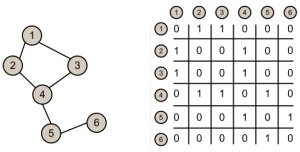
Let G = (V, E) represent a graph.

Let w : E -> W be a function that associates to each edge a cost (weight). If an edge does not exist between two nodes we assume a cost of +infinite.

Let numNodes represent the number of vertices in the graph.

Let numEdges represent the number of edges in the graph.

Let minDist[u] refer to an algorithm’s estimation of the minimum distance from the source to node u.

Let parent[u] refer to the second-to-last element on the minimum cost path from the source to node v.

The general problem asks us to find a path between two given nodes such that total sum of the weights is minimum.

Relaxing an edge

Relaxation of an edge (u, v) refers to improving the current estimation of the minimum cost for a path from the source node to node v by using the respective edge.

void relaxEdge (Vertex u, Vertex v)
{
    if (minDist[v] > minDist[u] + w(u, v)) {
        minDist[v] = minDist[u] + w(u, v);
        parent[v] = u;
    }
}

Single source shortest path problem

Given one source node, find the shortest path to all the other nodes in the graph. Ideally, we want to analyze each node/edge only once.

Scenarios:   

• The graph is undirected and acyclic (a tree)
  In this situation there is only one path from one node to another so we can find the answer with a depth first search.
  Time complexity: Θ (numNodes + numEdges)                                                                              

• The graph is a directed and acyclic (a DAG)
  For solving the problem we can explore each node in sorted topological order and apply the relaxEdge procedure for each corresponding edge. This approach requires only two traversals of the graph.
  Time complexity: Θ  (numNodes + numEdges)                                                                            
• A graph where each edge has an equal weight.
  For this scenario, the best approach is to apply the Breadth First Search algorithm. The order in which nodes are explored is given by the minimum number of edges from the source, which coincides with the shortest path.
  Time complexity: Θ  (numNodes + numEdges)                                                                                 
  • A graph with edges that have only positive weights.                                                                                                                
    When we extracted a node from the front of the queue during BFS, we had the guarantee that it was the closest unexplored node from the source, in terms of number of edges. If we change the problem so that edges have different but positive weights we need to replace the queue with another data structure that supports efficient interrogation for the closest node. This type of data structure is called a priority queue. We would also like to be able adjust the estimated value for a node efficiently, for when we relax an edge.
    The following algorithm is known as Dijkstra’s algorithm.

    
    // setup an initial distance estimation
    void initDistance(Graph, Vertex s)
    {
         for each Vertex v in Graph {
             minDist[v] = infinite;
             visited[v] = false;
         }
         // set minDist for source to 0
         minDist[s] = 0;
    }
    
    void Dijkstra(Graph, Vertex source)
    {
        initDistance(Graph, source);
        PriorityQueue PQ;
        PQ.add(source);
    
        while (!PQ.empty()) {
           // u is the closest unexplored node to the source
           Vertex u = PQ.extractMin();
           mark u as explored
    
           for each Vertex v that is connected to Vertex u {
               if Vertex v is not explored {
                   relaxEdge(v, u)
                   updatePQ(v);
                   // update PQ with the new estimation
                   // of distance for v
               }
          }
        }
    }
    

    For Java and C there already exist implementations for a priority queue data structure: PriorityQueue and priority_queue. These implementations have logarithmic time complexity for element addition and extraction, but don’t allow you to update the priority of a random element.

    Note that, since the priority queue will contain node references, to use these existing data structures you need to implement a comparator first and supply it to the constructor.

    The default Priority Queue in Java works as a min-heap (returns the minimum element, as indicated by the comparator), while the C++ equivalent data structure priority_queue is a max-heap (default behaviour is to return the maximum element).

    class NodeComparator implements Comparator
    {
        @Override
        public int compare(Vertex u, Vertex v) {
            return minDist[u.index] < minDist[v.index] ? 1 : -1;
        }
    }
    

    Complexity of Dijkstra’s algorithm

    We explore each node exactly once and this translates to one call to PQ.extractMin() for each node. We also only check each edge once, but in the worst case scenario we have to update the priority queue structure with each check.

    Therefore, we can express the complexity as:

    Θ (numNodes * Extract-Min + numEdges * UpdatePQ)

    The exact complexity of Dikstra’s algorithm depends on how we implement the priority queue:

    As a simple array:

    • Extract-Min: Θ (numNodes)
    • UpdatePQ: Θ (1)

    Time complexity: Θ (numNodes^2 + numEdges), which is efficient for dense graphs.

     As a binary heap:

    • Extract-Min: Ο( log(numNodes) )
    • UpdatePQ: Ο( log(numNodes) )

    Time complexity: Θ (numEdges * log(numEdges)), which is efficient for sparse graphs.

    As a Fibonacci heap:

    • Extract-Min: Ο( log(numNodes) )
    • UpdatePQ: Ο(1)*

    Time complexity: Θ (numNodes * log(numNodes) + numEdges)

    Possible exam questions

    • What is the order of exploration of the nodes, using Dijkstra’s algorithm, given a graph and a source node?
    • Why doesn’t Dijkstra work if we have negative weight edges? Think of a simple example.

     

• A graph with edges that have both negative and positive weights 
  For this scenario we may apply the Bellman Ford algorithm, where we basically relax each edge for numNodes-1 iterations:

  void BellmanFord(Graph, source)
  {
      initDistance(Graph, source);
      for (i = 1; i <= numNodes - 1; i++) {
          for each edge(u, v) in Graph {
              relax(u, v);
          }
      }
  }
  

  Complexity for Bellman Ford: Θ (numNodes * numEdges).

  Possible exam question:

  If it is still possible to relax an edge after we run Bellman-Ford than there exists a negative cycle in the graph.Why? Hint: How many iterations does it take to obtain the shortest distance for any destination in the worst case scenario?

Master Theorem examples

Because you have requested more examples for the Master Theorem, below are some further references:

[1] https://en.wikipedia.org/wiki/Master_theorem

[2] http://andrei.clubcisco.ro/cursuri/2aa/lab/lab4.pdf

[3] http://andrei.clubcisco.ro/cursuri/2aa/diverse/Exercitii%20teorema%20master.pdf

Starter Code (Lab)

(Last Edit 11.12.2015: Lab 4 Minimum Spanning Tree)

Beginning with the present lab, you may use the starter code found at this address:

[0] https://github.com/adcfils/assignments/archive/master.zip

 

Graph Representation – Quick Tutorial

Graphs are very powerful tools for modeling relations between various entities, with many applications in fields as diverse as physics, biology, networking, natural language processing, etc. In this post we are going to overlook the most common ways of representing graphs in memory.

Graphs are usually defined as an ordered pair G = (V, E) where

• V represents the set of vertices or nodes
• E represents the set of edges, an edge being a link between two vertices

Depending on the problem, a graph or it’s components may have various properties (such as having directed or undirected edges), but every graph implementation should generally provide an implementation for:

• adding a node or an edge
• checking if an edge exists between two nodes
• traversing every edge associated with a node
• (optionally) deleting a node or an edge

There are two common ways to model graphs in memory: using adjacency lists or an adjacency matrix.

Using an Adjacency Matrix

• Building the graph

If we have prior knowledge of the total number of nodes in the graph, building the graph becomes as simple as:

void initGraph(int numNodes) {
     matrix = new boolean[numNodes][numNodes];
     vertices = new Vertex[numNodes];
}

Here matrix[i][j] has the value 1 if there exists an edge from node i to node j and 0 otherwise.

The space required for storing the matrix amounts to Θ (numNodes^2). Depending on usage, we may decide to store additional information for each vertex or edge. For example, here we assume each Vertex object holds an index variable.
Note that, in practice, this representation becomes entirely unfeasible for larger graphs. For example, a typical graph holding around ~1.000.000 nodes would require as much as 1 Terabyte for the matrix alone (or 125 GB if we opt out for a BitSet representation)!
Moreover, adding new nodes at runtime may involve copying the contents of the old matrix onto an entirely new matrix of different size.

• Adding an edge

void addEdge(Vertex v, Vertex u) {
     matrix[v.index][u.index] = true;
}

This method adds a link between vertex v and u in constant time. If the graph is undirected, the corresponding value between vertex u and v must also be set to true. Similarly, checking and removing edges translates to simple table lookups, with constant time complexity:

• Check if an edge exists between two nodes

boolean checkEdge(Vertex v, Vertex u) {
     return matrix[v.index][u.index];
}

• Remove an edge between two nodes

boolean removeEdge(Vertex v, Vertex u) {
     matrix[v.index][u.index] = false;
}

• Traverse every edge associated with a node

Many algorithms require that we iterate through every neighbour of a particular node and apply some specific computation. For finding the set of neighbours, this representation forces us to go, each time, over every node in the graph and to check if an edge exists.

The time complexity becomes Θ(numNodes) per each call or Θ(numNodes^2) if we want to traverse the whole graph:

void computeForEachNeighbour(Vertex v, Consumer computation){
     for (int i = 0; i < this.numNodes; ++i) {
          if (checkEdge(v, vertices[i])) {
               // do some computation with this vertex
               computation.accept(vertices[i]);
          }
     }
}

Using adjacency lists

• Building the graph

This approach builds, for each separate vertex, a list of valid edges. Thus, the total space required grows linearly in size with the number of nodes and edges in the graph: Θ(numNodes+numEdges). This makes it possible to store large yet sparse graphs.

void initGraph(int numNodes) {
     vertices = new ArrayList<ArrayList<Vertex>>(numNodes);
}

• Adding an edge

Adding an edge or a node requires constant time.

void addEdge(Vertex v, Vertex u) {
     this.vertices.get(v.index).add(u);
}

• Traverse every edge associated with a node

This time, checking every edge leaving a node is more efficient because we only touch valid edges. Time complexity is Θ (k), where k is the number of neighbours, or Θ (numNodes + numEdges) if you want to traverse the whole graph.

void computeForEachNeighbour(Vertex v, Consumer function){
     for (Vertex u : vertices.get(v.index)) {
          // apply some computation on the vertex
          function.accept(u); 
     }
}

Note that checking if an edge exists between two nodes requires a call to this function and thus it’s time complexity is Θ (numEdges) and likewise for deleting an edge.

Conclusion

• Adjacency Matrix

Space required for storing the graph: Θ (numNodes^2)
Time for checking if an edge exists: Θ (1)
Time for adding/removing an edge: Θ (1)
Time for traversing every edge: Θ (numNodes^2)
This approach is recommended for small graphs that either have many edges or require frequent edge modifications and lookups at run-time.

• Adjacency Lists

Space required for storing the graph: Θ (numNodes + numEdges)
Time for checking if an edge exists: Ο (numEdges)
Time for adding an edge: Θ (1)
Time for removing an edge: Ο (numEdges)
Time for iterating over every edge: Θ (numNodes+numEdges)
This approach is better suited for graphs that have relatively few edges, making it a preferable choice for many real-world problems.

In conclusion, there is no general “correct” implementation, as each solution must take into account the type of graph and the expected usage pattern for the lookup methods.

[0] http://java.dzone.com/articles/algorithm-week-graphs-and

Divide and Conquer Laboratory

I have uploaded the problems from the Divide and Conquer laboratory.

Laboratory 2

Complexity Laboratory

I have attached a pdf with the exercies that we have done at the complexity seminar.

Laboratory 1

Lab 6

1. Compute the minimum spanning tree of a given graph using Kruskal’s algorithm.

2. Find the shortest path in a graph from a given source node to a given destination using Dijkstra’s algorithm.

Lab 5 Applications for DFS

1. Find the strongly connected components of a given graph.

2. Find the articulation points of a given graph.

Lab 4 Graph Search Algorithms

1. Check if a directed graph is cyclic, using DFS.

2. Given a m*n cell maze with two kinds of cells: empty and obstacle, a source cell and a destination cell, find the shortest path from source to destination, using BFS.

Lab 3 Dynamic Programming

1. Find the maximum contiguous subsequence sum in an array of integers.

2. Consider a row of n coins of values v(1) …v(n), where n is even. We play a game against an opponent by alternating turns. In each turn, a player selects either the first or last coin from the row, removes it from the row permanently, and receives the value of the coin. Determine the maximum possible amount of money we can definitely win if we move first. (Consider the other player is smart and makes the best choice.)